Central limit theorem: simulate what actually converges
In this article (7 sections)
In the classical independent, identically distributed setting with finite nonzero variance, the central limit theorem describes the limiting distribution of the standardized sample mean. It does not say that the original observations become normally distributed as you collect more of them.
The distinction is easier to see when the population is clearly skewed. This original simulation uses an exponential distribution with mean two and standard deviation two.
Standardize the quantity of interest
For a sample of size n, calculate its mean, subtract the population mean two and divide by the theoretical standard error 2 / sqrt(n). Equivalently, Z = sqrt(n) × (sample_mean - 2) / 2.
Under the stated assumptions, Z approaches a standard normal distribution as n grows. The unstandardized mean simultaneously becomes more concentrated around two.
MIT's LLN and CLT reading provides the theorem context. The exponential simulations and figures here are original, with recorded seeds and actual execution results.
Inspect repeated samples, not one mean
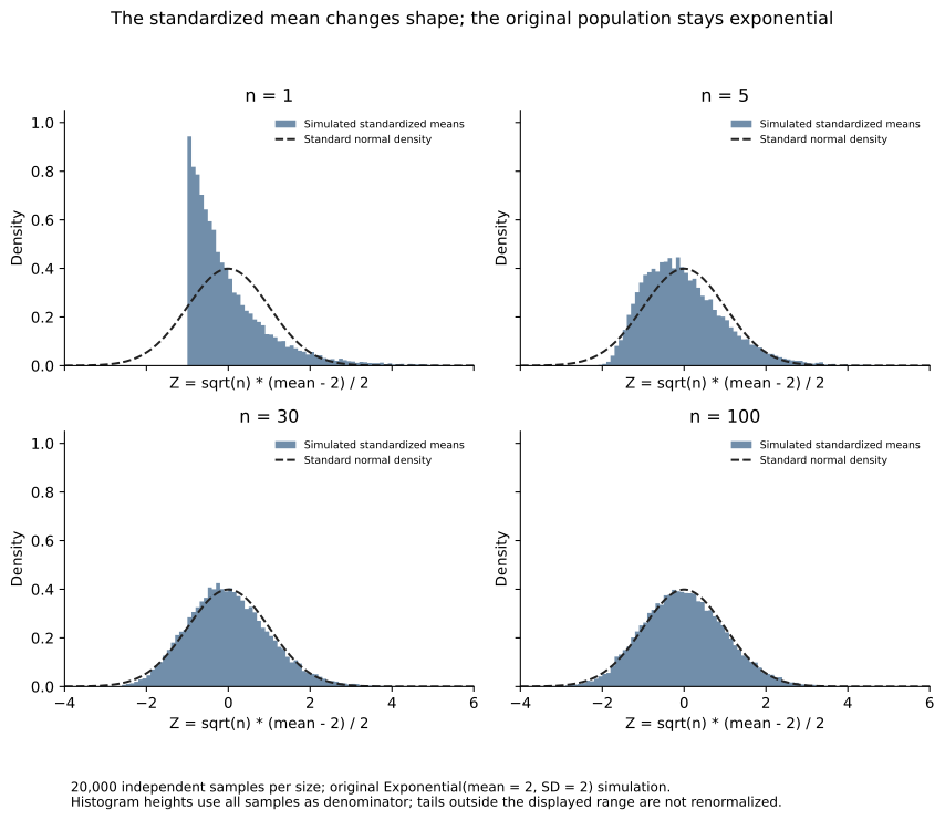
Open the full-size SVG for zooming. Each panel contains 20,000 independent samples of the specified size.
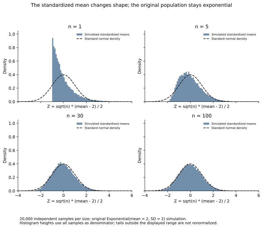
The n=1 panel is strongly skewed. At n=100 the standardized distribution is closer to normal, although finite-sample skew remains. The plot uses all simulation samples in its histogram denominator; the small tail outside the displayed range is not renormalized away.
Reproduce the numerical checks
import numpy as np
from sampling_limits import summarize,repeated_means

report = summarize()
rows = report['independent_repeated_samples']
assert [r['n'] for r in rows]==[1,5,30,100]
assert all(r['repetitions']==20000 for r in rows)
for r in rows:
    assert abs(r['z_mean'])<.04
    assert abs(r['z_sd_ddof1']-1)<.04
    assert np.isclose(r['sd_of_means_ddof1'],r['z_sd_ddof1']*2/np.sqrt(r['n']))
assert rows[-1]['z_skewness_bias_false']<rows[0]['z_skewness_bias_false']
assert np.array_equal(repeated_means(30),repeated_means(30))
print([{k:r[k] for k in ['n','sd_of_means_ddof1','z_sd_ddof1','z_skewness_bias_false']}
       for r in rows])
The sampling lab records the generator configuration and runtime. Seeds are integers defined by 20260929 + n; they identify runs and are not calendar dates.
Read the two scales separately
| Sample size | Observed SD of means | Observed standardized skewness |
|---|---|---|
| 1 | 2.0171 | 2.0372 |
| 5 | 0.8933 | 0.8940 |
| 30 | 0.3661 | 0.3802 |
| 100 | 0.2016 | 0.1994 |
The SD of the unstandardized means shrinks, while the standardized SD remains near one. Standardization removes the shrinking scale so the changing distributional shape can be inspected.
These values are finite simulation results, not exact theorem constants or evidence that every future run must produce the same empirical moments under a different runtime or seed.
Avoid the n=30 shortcut
There is no universal sample size at which every distribution becomes adequately normal for every purpose. Population shape, tails, dependence and the probability region of interest affect approximation quality.
The n=30 exponential example still has visible positive skew. A central approximation may be useful while a tail probability needs more care. Evaluate the approximation for the actual decision rather than relying on a memorized threshold.
Check the assumptions before using the result
Duplicated observations do not provide independent information merely because the row count is large. The lab includes a perfect-dependence example in which one draw is repeated one hundred times; averaging those copies does not produce the independent-sample precision gain.
Distributions without the finite-variance conditions of this classical theorem require different treatment. A simulation that looks roughly bell-shaped is not a proof that all assumptions are satisfied.
Exercise: plot the raw exponential observations beside the n=100 sample means. Explain why the raw-data histogram remains skewed and why the mean histogram has a different spread and shape.
NeuraPath's Data Science course connects probability theory with reproducible statistical reasoning. Understanding what converges helps you use normal approximations without turning the CLT into an unsupported claim about the raw data.
Continue learning
This article is part of the Mathematics and statistical foundations sequence. Use the neighbouring tasks when you need the prerequisite or the next application.
- Review the prerequisite or neighbouring task in Bayes' theorem: update a probability without ignoring the base rate.
- Continue with Law of large numbers versus central limit theorem.
Pankit Kumar has 10 years in Data Science & AI, building and shipping production systems in regulated pharma and clinical environments. He is a freelance trainer at Boston Institute of Analytics, AnalytixLabs and Scaler, and has taught this material to thousands of working professionals.
This article is part of our Data Science programme — 6 months. From data foundations to machine learning, deep learning and deployment.
Explore Data Science